An Exploration of Feature Selection and Machine Learning Algorithms
This writeup is an extension of a Master’s thesis project I completed in 2022 for an advanced Machine Learning course. Essentially, I intended to do a thorough but non-exhaustive exploration of feature selection algorithns, both simple and complex, in conjunction with ML algorithms for classification tasks. I present it here as a broad view of how trial-and-error approaches can be useful in designing ML pipelines and for presenting some reliable template code for conducting ML in Python 3.
The dataset used in this project is a common one for classification tasks: the BRFSS Arthritis dataset made available by the CDC. The version of the data used in this project comes from 2018. It is a large dataset with many numerical and categorical factors, as well as a target variable for arthritis diagnosis.
This project was initially completed in this Collab notebook.
Data Preprocessing
After examining the dataset (block 1 of my coding document), I found a few key areas of preprocessing to focus on. First, while all values appeared to be numerical, some values were encoded as string type instead of a numeric type. In block 2 of my coding document, I forced all values to be numeric. Importantly, missing or NA values were not handled consistently in the dataset. Some columns contained ‘?’ symbols to represent missing data, whereas others had blanks or NA values. So, I replaced all ‘?’ instances with numpy’s Not-A-Number value (np.nan). Then, I used the median of each column to replace any np.nan instances so that all values would be properly handled. I also noticed that the havarth3 column was encoded in a way that could be misleading for my classification methods. I prefer when a 1 represents a positive instance and a 0 represents a negative instance, which is also how the scikit-learn suite handles class attributes. So, I changed that last column, transforming all 2’s into 0’s, since they represented negative cases of arthritis. One preprocessing step that I considered but ultimately decided not to do was eliminating redundant columns. There are several columns that encode age in different ways, which felt like it might confuse a classification algorithm. I decided not to eliminate any columns because the Codebook demonstrated that there was no one column that appeared to be better for classification than any other. For example, the strict Age column (called DIABAGE2) has 376,733 missing values. The other age columns are categorical (encoded numerically), but they have fewer missing values. Selecting the “best” age column felt arbitrary and ultimately unhelpful. A similar train of thought applies for many other columns in this large dataset. Values of height and weight are strangely encoded depending on their unit of measurement. Rather than agonize over which columns to keep and which to eliminate for purposes of classification, I decided to keep all columns and hope that the sophistication of the attribute selection and classification algorithms would be sufficient to produce decently accurate results. It should be noted that some attribute selection methods did get confused by these redundant columns, which may have had a detrimental impact on their performance.
The code segments below show the initial data preprocessing steps:
Data Import
import pandas as pd
import warnings
warnings.filterwarnings('ignore') #ignore warnings
import numpy as np
import seaborn as sns
pd.set_option('display.expand_frame_repr', False) #view many columns at once

url = 'https://raw.githubusercontent.com/ethanperitz/datasets/main/project-2018-BRFSS-arthritis.csv'
df = pd.read_csv(url)
df.head()
Data Cleaning
for column in list(df.columns):
  current_column = df[column]
  current_column = current_column.replace('?', np.nan) #replaces question marks with nan
  current_column = pd.to_numeric(current_column) #forces columns to numeric datatype
  current_median = current_column.median() #get median of column to replace nan values
  current_column = current_column.fillna(current_median) #replace nan with median
  df[column] = current_column #set new column

#We want arthritis values to be 1 and non-arthritis values to be 0 for simple interpretation of classifier models.
df['havarth3'] = np.where(df['havarth3'] == 1, 1, 0)
df.head()
Train and Test Data Definitions
from sklearn.model_selection import train_test_split

#prepare column lists, x and y (class attribute)
y = df['havarth3'].values
list_of_columns = list(df.columns)
list_of_columns.remove(list_of_columns[-1])
X = df[list_of_columns].values

#split with stratification

X_train, X_test, y_train, y_test = train_test_split(X, y, \
                                                    test_size=0.34, \
                                                    stratify=y, \
                                                    random_state=47)
Feature/Attribute Selection
Perhaps the most important question in ML: How does one select the data features that will produce accurate and consistent classifications? If this question were easy to answer, Data Science would not be held in such regard. I find that patience, trial-and-error, and a good understanding of your data structures go a very long way. Here are 5 attribute selection methods you might use.
Attribute Selection #1: Pearson Correlation Values
For my first method, I created a correlation matrix of all attributes, then selected the ten attributes with the strongest Pearson correlation coefficients with the class attribute (havarth3). The selected attributes are copied below: ‘x.age80’, ‘x.age.g’, ‘x.ageg5yr’, ‘employ1’, ‘genhlth’, ‘x.hcvu651’, ‘x.age65yr’, ‘diffwalk’, ‘rmvteth4’, ‘x.phys14d’ We can see that this method was confused by the multiple Age columns.
Attribute Selection #2: Chi Square
I used chi square p-values to find attributes that had an association with the class attribute. Initially, I thought that I would select the attributes with the 10 smallest p-values, but I then found that there were 18 attributes whose p-values were so small that python reported them as 0. Rather than pick and choose from among these, I simply selected all 18. These attributes are printed below: ‘employ1’, ‘weight2’, ‘height3’, ‘children’, ‘alcday5’, ‘physhlth’, ‘wtkg3’, ‘x.bmi5’, ‘x.age80’, ‘x.ageg5yr’, ‘x.drnkwek’, ‘drocdy3.’, ‘x.llcpwt2’, ‘x.llcpwt’, ‘x.wt2rake’, ‘x.ststr’, ‘x.strwt’, ‘x.hcvu651’
Attribute Selection #3: Mutual Information Gain
I selected the ten attributes that had the highest mutual information gain with the class attribute. These attributes are printed below: ‘x.age80’, ‘x.ageg5yr’, ‘x.age.g’, ‘employ1’, ‘diffwalk’, ‘pneuvac4’, ‘x.rfhlth’, ‘x.age65yr’, ‘x.hcvu651’, ‘x.phys14d’
Attribute Selection #4: Recursive Feature Elimination
While not covered in this class, I found through my own reading that recursive feature elimination is a popular algorithm for attribute selection, as it considers each attribute, ranks it in accordance with how helpful it will be as a classifier, and then eliminates any attributes found to be unhelpful. It recursively repeats this process until a desired number of attributes are remaining. This process took a surprisingly long amount of time to run – around 15 minutes – and I ended up with the following attributes: ‘weight2’, ‘height3’, ‘alcday5’, ‘x.psu’, ‘wtkg3’, ‘x.drnkwek’, ‘drocdy3.’, ‘x.llcpwt2’, ‘x.llcpwt’, ‘x.ststr’ As a side note, I will say that this method did not appear to work well at all. It selected an attribute with hidden values (ststr) and other attributes that appear to have very little correlation with the class attribute.
Attribute Selection #5: Difference in Means
For the last attribute selector, I found the difference in means for each column between tuples classified with Arthritis and those classified without Arthritis. I standardized the values so that the scales would not be a factor, and I took the fifteen largest differences in means. Originally, I had selected the ten largest differences, but I realized that the group of attributes was identical to those selected from method #1 (Pearson correlations). So, for variety, I added the next five largest differences. The list of attributes is printed below: ‘x.age80’, ‘x.age.g’, ‘x.ageg5yr’, ‘employ1’, ‘genhlth’, ‘x.hcvu651’, ‘x.age65yr’, ‘diffwalk’, ‘rmvteth4’, ‘x.phys14d’, ‘x.rfhlth’, ‘physhlth’, ‘children’, ‘pneuvac4’, ‘qstver’
Modeling with ML Algorithms
For each of the 5 feature selection algorithms, I enmployed the following classifier methods:
Classifier #1: Naïve Bayes
Naïve Bayes assumes independence of features and finds the highest probability of each value of the class attribute under the condition of each distinct value in each tuple. Naïve Bayes tends to work well with categorical attributes, and since there are some numerical attributes in the dataset, I used the Gaussian Naïve Bayes provided by scikit-learn.
Classifier #2: k-Nearest Neighbors
The KNN algorithm calculates Euclidean distances on an n-dimensional hyperplane for each new tuple and classifies it according to a simple majority of nearby points. In other words, if k = 5, and the three of the five closest points to an unclassified point are Class 1, we predict that the unclassified point is Class 1.
Classifier #3: Logistic Regression
This approach classifies using a sigmoid function and a threshold for probability. Values of the sigmoid function greater than the threshold are classified one way, and all other values are classified in the other way.
Classifier #4: Decision Tree
This classification method uses information gain to create efficient decision trees whose depth continues until the highest level of purity has been achieved. The default metric for information gain is the Gini index.
Classifier #5: Random Forest
This method is similar to #4 above, but it is an ensemble method that creates many different Decision Trees that expand to a given maximum depth, then chooses the Decision Tree that had the best accuracy. For all methods above, I used a python implementation and the appropriate scikit-learn packages.
Code Example
Rather than copy all of the code written for this project here, I will include just one example of a feature selection / classifier pair. For all the others (which each have their own nuances, hyperparameters, etc.), the reader is invited to examine the Collab document.
Feature Selection Algorithm: Pearson’s R
cor = df.corr() #create correlation matrix
cor = cor[cor['havarth3'] < 1] #remove self-correlation
target = cor['havarth3'] #isolate class attribute's correlation values
target = abs(target) #take absolute values
features = target.nlargest(10) #find 10 strongest correlations
selected_features = list(features.index)
print(selected_features)
attr1_X_train = train_df[selected_features] #filter X_train
attr1_X_test = test_df[selected_features] #filter X_test
ML Classifier: Naive Bayes
#Naive Bayes
print('NAIVE BAYES\n')
from sklearn.preprocessing import StandardScaler
from sklearn.naive_bayes import GaussianNB
from sklearn import metrics
from sklearn.metrics import confusion_matrix

#scale
s = StandardScaler()
X_train = s.fit_transform(attr1_X_train)
X_test = s.fit_transform(attr1_X_test)

#fit model
gnb = GaussianNB()
y_pred = gnb.fit(X_train, y_train).predict(X_test)

#performance measures
acc = metrics.accuracy_score(y_test, y_pred)
tn, fp, fn, tp = confusion_matrix(y_test, y_pred).ravel()
print(f'Accuracy of Classifier:  {round(acc, 4)}\n')
print(f' True Positives = {tp}\n True Negatives = {tn}\n \
False Positives = {fp}\n False Negatives = {fn}\n \
True Positive Rate (Sensitivity/Recall) = {round(tp/(tp+fn), 4)}\n \
True Negative Rate (Specificity) = {round(tn/(tn+fp), 4)}\n \
F-Measure = {round(metrics.f1_score(y_test, y_pred), 4)}\n \
ROC Area Under Curve = {round(metrics.roc_auc_score(y_test, y_pred),4)}\n \
MCC = {round(metrics.matthews_corrcoef(y_test, y_pred), 4)}')
Notice how evaluation metrics are built directly into the coding structure - an extremely important inclusion. Below is the output from this example:
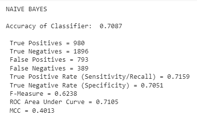
Summary
These classification procedures had mixed results. In general, models were better at correctly predicting when people would not develop arthritis than they were at predicting when people would develop arthritis. A few models, though, performed well for both. Broadly, Naïve Bayes did the best job in terms of accurate predictions and low variation between the true positive rate and the true negative rate. And, as we would expect, the Random Forest Classifier always outperformed the Decision Tree Classifier by a small margin. The most inconsistent results came from the k-Nearest Neighbors classifiers and the Logistic Regression classifiers. Often, their overall accuracy was decent, but they performed much better on one class than the other. One result – the Logistic Regression for Recursive Feature Elimination – did a terrible job at classifying people with arthritis (5% TPR) and an excellent job at classifying people without arthritis (98% TNR). As stated earlier, the Recursive Feature Elimination’s attribute selections were very strange, which is probably a factor of the repetitive and inconsistent columns in the original dataset. All five models created for these attributes underperformed all others of the same type, which gives credence to the “garbage in – garbage out” heuristic. Interestingly, the attribute selection methods that did the best were also the simplest. Pearson correlation and difference in means produced very similar sets of attributes, and these attributes performed the best on the classification algorithms. So, one important takeaway from this project is that complex is not always better. I also learned that Naïve Bayes appears to be quite robust even when the independence of features condition is violated. It performed well even when fed features that were certainly not independent of each other (as many body measurement variables are quite dependent on each other).
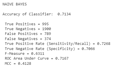
Best Feature Selection / Classifier Pair
The best performer was a Naive Bayes classifier that utilized a simple Difference in Means feature selection algorithm. The evaluation is shown below:
Students in ML classes should expect to practice with these algorithms often, both in implementation and in explanation. Over time, you start to learn how algorithms behave in certain circumstances and how to create effective ensemble-based algorithms and iterate on past results. Happy Machine Learning!